Inner Stabilization
The mission of this script is to process data from Mirnov coils, determine plasma position and thus help with plasma stabilization. Mirnov coils are type of magnetic diagnostics and are used to the plasma position determination on GOLEM. 4 Mirnov coils are placed inside the tokamak 93 mm from the center of the chamber. The effective area of each coil is $A_{eff}=3.8\cdot10^{-3}$ m. Coils mc9 and mc1 are used to determination the horizontal plasma position and coils mc5 and mc13 to determination vertical plasma position.
 |
Procedure (This notebook to download)
import os
import glob

#remove files from the previous discharge
def remove_old(name):
    if os.path.exists(name):
        os.remove(name)

names = ['analysis.html','icon-fig.png', 'plasma_position.png']
for name in names:
    remove_old(name)

if os.path.exists('Results/'):
    file=glob.glob('Results/*')
    for f in file:
        os.remove(f)

import numpy as np
import matplotlib.pyplot as plt

from scipy import integrate, signal, interpolate
import pandas as pd


import holoviews as hv
hv.extension('bokeh')
import hvplot.pandas
import requests

from IPython.display import Markdown

#execute time
from timeit import default_timer as timer
start_execute = timer()


BDdata_URL = "http://golem.fjfi.cvut.cz/shots/{shot_no}/Diagnostics/BasicDiagnostics/{identifier}.csv"
data_URL = "http://golem.fjfi.cvut.cz/shots/{shot_no}/Diagnostics/LimiterMirnovCoils/DAS_raw_data_dir/NIdata_6133.lvm" #NI Standart (DAS) new address


shot_no = 36070 # to be replaced by the actual discharge number
# shot_no = 35940
vacuum_shot = 36038 # to be replaced by the discharge command line paramater "vacuum_shot"
# vacuum_shot = 35937 #number of the vacuum shot or 'False'

ds = np.DataSource(destpath='')
def open_remote(shot_no, identifier, url_template=data_URL):
    return ds.open(url_template.format(shot_no=shot_no, identifier=identifier))

def read_signal(shot_no, identifier, url = data_URL, data_type='csv'):
    file = open_remote(shot_no, identifier, url)
    if data_type == 'lvm':
        channels = ['Time', 'mc1', 'mc5', 'mc9', 'mc13', '5', 'RogQuadr', '7', '8', '9', '10', '11', '12']
        return pd.read_table(file, sep = '\t', names=channels)
    else:
        return pd.read_csv(file, names=['Time', identifier],
                     index_col = 'Time', squeeze=True)
Data integration and $B_t$ elimination
The coils measure voltage induced by changes in poloidal magnetic field. In order to obtain measured quantity (poloidal magnetic field), it is necessary to integrate the measured voltage and multiply by constant: $B(t)=\frac{1}{A_{eff}}\int_{0}^{t} U_{sig}(\tau)d\tau$
Ideally axis of the coils is perpendicular to the toroidal magnetic field, but in fact they are slightly deflected and measure toroidal magnetic field too. To determine the position of the plasma, we must eliminate this additional signal. For this we use vacuum discharge with the same parameters.
def elimination (shot_no, identifier, vacuum_shot = False):
    #load data
    mc = (read_signal(shot_no, identifier, data_URL, 'lvm'))
    mc = mc.set_index('Time')
    mc = mc.replace([np.inf, -np.inf, np.nan], value = 0)
    mc = mc[identifier]

    konst = 1/(3.8e-03)


    if vacuum_shot == False:
        signal_start = mc.index[0]
        length = len(mc)
        Bt = read_signal(shot_no, 'BtCoil_integrated', BDdata_URL).loc[signal_start:signal_start+length*1e-06]
        if len(Bt)>len(mc):
            Bt = Bt.iloc[:length]
        if len(Bt)<len(mc):
            mc = mc.iloc[:len(Bt)]

        if identifier == 'mc1':
            k=300
        elif identifier == 'mc5':
            k= 14
        elif identifier == 'mc9':
            k = 31
        elif identifier == 'mc13':
            k = -100

        mc_vacuum = Bt/k
    else:
        mc_vacuum = (read_signal(vacuum_shot, identifier, data_URL, 'lvm'))
        mc_vacuum = mc_vacuum.set_index('Time')
        mc_vacuum = mc_vacuum[identifier]
        mc_vacuum -= mc_vacuum.loc[:0.9e-3].mean()    #remove offset
        mc_vacuum = mc_vacuum.replace([np.inf, -np.inf], value = 0)

        mc_vacuum = pd.Series(integrate.cumtrapz(mc_vacuum, x=mc_vacuum.index, initial=0) * konst,
                    index=mc_vacuum.index*1000, name= identifier)    #integration

    mc -= mc.loc[:0.9e-3].mean()  #remove offset

    mc = pd.Series(integrate.cumtrapz(mc, x=mc.index, initial=0) * konst,
                    index=mc.index*1000, name= identifier)    #integration

    #Bt elimination
    mc_vacuum = np.array(mc_vacuum)
    mc_elim = mc - mc_vacuum

    return mc_elim
Plasma life time
loop_voltage = read_signal(shot_no, 'U_Loop', BDdata_URL)
dIpch = read_signal(shot_no, 'U_RogCoil', BDdata_URL)

dIpch -= dIpch.loc[:0.9e-3].mean()

Ipch = pd.Series(integrate.cumtrapz(dIpch, x=dIpch.index, initial=0) * (-5.3*1e06),
                index=dIpch.index, name='Ipch')

U_l_func = interpolate.interp1d(loop_voltage.index, loop_voltage)
def dIch_dt(t, Ich):
    return (U_l_func(t) - 0.0097 * Ich) / (1.2e-6/2)
t_span = loop_voltage.index[[0, -1]]
solution = integrate.solve_ivp(dIch_dt, t_span, [0], t_eval=loop_voltage.index, )
Ich = pd.Series(solution.y[0], index=loop_voltage.index, name='Ich')
Ip = Ipch - Ich
Ip.name = 'Ip'

Ip_detect = Ip.loc[0.0025:]

dt = (Ip_detect.index[-1] - Ip_detect.index[0]) / (Ip_detect.index.size)

window_length = int(0.5e-3/dt)
if window_length % 2 == 0:
    window_length += 1
dIp = pd.Series(signal.savgol_filter(Ip_detect, window_length, polyorder=3, deriv=1, delta=dt),
                name='dIp', index=Ip_detect.index) / 1e6

threshold = 0.05

CD = requests.get("http://golem.fjfi.cvut.cz/shots/%i/Production/Parameters/CD_orientation" % shot_no)
CD_orientation = CD.text

if "ACW" in CD_orientation:
    plasma_start = dIp[dIp < dIp.min()*threshold].index[0]*1e3
    plasma_end = dIp.idxmax()*1e3
else:
    plasma_start = dIp[dIp > dIp.max()*threshold].index[0]*1e3
    plasma_end = dIp.idxmin()*1e3 + 0.5


print ('Plasma start =', round(plasma_start, 3), 'ms')
print ('Plasma end =', round(plasma_end, 3), 'ms')
# print (CD_orientation)
Plasma Position
To calculate displacement of plasma column, we can use approximation of the straight conductor. If we measure the poloidal field on the two opposite sides of the column, its displacement can be expressed as: $\Delta=\frac{B_{\Theta=0}-B_{\Theta=\pi}}{B_{\Theta=0}+B_{\Theta=\pi}}\cdot b$
Horizontal plasma position $\Delta r$ calculation
def horpol(shot_no, vacuum_shot=False):
    mc1 = elimination(shot_no, 'mc1', vacuum_shot)
    mc9 = elimination (shot_no, 'mc9', vacuum_shot)

    b = 93

    r = ((mc1-mc9)/(mc1+mc9))*b
    r = r.replace([np.nan], value = 0)

#     return r.loc[plasma_start:]
    return r.loc[plasma_start:plasma_end]
#     return r
r = horpol(shot_no, vacuum_shot)
ax = r.plot()
ax.set(ylim=(-85,85), xlim=(plasma_start,plasma_end), xlabel= 'Time [ms]', ylabel = '$\Delta$r [mm]', title = 'Horizontal plasma position #{}'.format(shot_no))
ax.axhline(y=0, color='k', ls='--', lw=1, alpha=0.4)

Vertical plasma position $\Delta z$ calculation
def vertpol(shot_no, vacuum_shot = False):
    mc5 = elimination(shot_no, 'mc5', vacuum_shot)
    mc13 = elimination (shot_no, 'mc13', vacuum_shot)

    b = 93

    z = ((mc5-mc13)/(mc5+mc13))*b
    z = z.replace([np.nan], value = 0)
#     return z.loc[plasma_start:]
    return z.loc[plasma_start:plasma_end]
#     return z
z = vertpol (shot_no, vacuum_shot)
ax = z.plot()
ax.set(ylim=(-85, 85), xlim=(plasma_start,plasma_end), xlabel= 'Time [ms]', ylabel = '$\Delta$z [mm]', title = 'Vertical plasma position #{}'.format(shot_no))
ax.axhline(y=0, color='k', ls='--', lw=1, alpha=0.4)

Plasma column radius $a$ calculation
def plasma_radius(shot_no, vacuum_shot=False):
    r = horpol(shot_no, vacuum_shot)
    z = vertpol(shot_no, vacuum_shot)

    a0 = 85
    a = a0 - np.sqrt((r**2)+(z**2))
    a = a.replace([np.nan], value = 0)
#     return a.loc[plasma_start:]
    return a.loc[plasma_start:plasma_end]
#     return a
a = plasma_radius(shot_no,vacuum_shot)
ax = a.plot()
ax.set(ylim=(0,85), xlim=(plasma_start,plasma_end), xlabel= 'Time [ms]', ylabel = '$a$ [mm]', title = 'Plasma column radius #{}'.format(shot_no))

plasma_time = []
t = 0
for i in a:
    if i>85 or i <0:
        a = a.replace(i, value = 0)
    else:

        plasma_time.append(a.index[t])

    t+=1
start = plasma_time[0]-1e-03
end = plasma_time[-1]-1e-03
print('start =', round(start, 3), 'ms')
print('end =', round(end, 3), 'ms')
Data
r_cut = r.loc[start:end]
a_cut = a.loc[start:end]
z_cut = z.loc[start:end]

df_processed = pd.concat([r_cut.rename('r'), z_cut.rename('z'), a_cut.rename('a')], axis= 'columns')
df_processed
savedata = 'plasma_position.csv'
df_processed.to_csv(savedata)
Markdown("[Plasma position data - $r, z, a$ ](./{})".format(savedata))
Graphs
hline = hv.HLine(0)
hline.opts(color='k',line_dash='dashed', alpha = 0.4,line_width=1.0)

layout = hv.Layout([df_processed[v].hvplot.line(
       xlabel='', ylabel=l,ylim=(-85,85), xlim=(start,end),legend=False, title='', grid=True, group_label=v)
                        for (v, l) in [('r', ' r [mm]'), ('z', 'z [mm]'), ('a', 'a [mm]')] ])*hline

plot=layout.cols(1).opts(hv.opts.Curve(width=600, height=200),  hv.opts.Curve('a', xlabel='time [ms]'))

plot
Results
df_processed.describe()
z_end=round(z_cut.iat[-25],2)
z_start=round(z_cut.iat[25],2)
r_end=round(r_cut.iat[-25],2)
r_start=round(r_cut.iat[25],2)

name=('z_start', 'z_end', 'r_start', 'r_end')
values=(z_start, z_end, r_start, r_end)
data={'Values':[z_start, z_end, r_start, r_end]}
results=pd.DataFrame(data, index=name)

dictionary='Results/'
j=0
for i in values :
    with open(dictionary+name[j], 'w') as f:
        f.write(str(i))
    j+=1

results
Icon fig
responsestab = requests.get("http://golem.fjfi.cvut.cz/shots/%i/Production/Parameters/PowSup4InnerStab"%shot_no)
stab = responsestab.text

if not '-1' in stab or 'Not Found' in stab and exStab==False:
    fig, axs = plt.subplots(4, 1, sharex=True, dpi=200)
    dataNI = (read_signal(shot_no, 'Rog', data_URL, 'lvm')) #data from NI
    dataNI = dataNI.set_index('Time')
    dataNI = dataNI.set_index(dataNI.index*1e3)
    Irog = dataNI['RogQuadr']
#     Irog=abs(Irog)
    Irog*=1/5e-3
    r.plot(grid=True, ax=axs[0])
    z.plot(grid=True, ax=axs[1])
    a.plot(grid=True, ax=axs[2])
    Irog.plot(grid=True, ax=axs[3])
    axs[3].set(xlim=(start,end), ylabel = 'I [A]')
    axs[2].set(ylim=(0,85), xlim=(start,end), xlabel= 'Time [ms]', ylabel = '$a$ [mm]')
    axs[1].set(ylim=(-85,85), xlim=(start,end), xlabel= 'Time [ms]', ylabel = '$\Delta$z [mm]')
    axs[0].set(ylim=(-85,85), xlim=(start,end), xlabel= 'Time [ms]', ylabel = '$\Delta$r [mm]',
               title = 'Horizontal, vertical plasma position and radius #{}'.format(shot_no))

else:
    fig, axs = plt.subplots(3, 1, sharex=True, dpi=200)
    r.plot(grid=True, ax=axs[0])
    z.plot(grid=True, ax=axs[1])
    a.plot(grid=True, ax=axs[2])
    axs[2].set(ylim=(0,85), xlim=(start,end), xlabel= 'Time [ms]', ylabel = '$a$ [mm]')
    axs[1].set(ylim=(-85,85), xlim=(start,end), xlabel= 'Time [ms]', ylabel = '$\Delta$z [mm]')
    axs[0].set(ylim=(-85,85), xlim=(start,end), xlabel= 'Time [ms]', ylabel = '$\Delta$r [mm]',
               title = 'Horizontal, vertical plasma position and radius #{}'.format(shot_no))

plt.savefig('icon-fig')

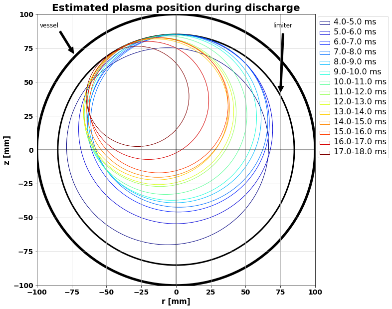
Plasma position during discharge
tms = np.arange(np.round(plasma_start),np.round(plasma_end)-1,1)

circle1 = plt.Circle((0, 0), 100, color='black', fill = False, lw = 5)
circle2 = plt.Circle((0, 0), 85, color='black', fill = False, lw = 3)

fig, ax = plt.subplots(figsize = (10,10))
ax.axvline(x=0, color = 'black', alpha = 0.5)
ax.axhline(y=0, color = 'black', alpha = 0.5)

ax.set_xlim(-100,100)
ax.set_ylim(-100,100)
ax.add_patch(circle1)
ax.add_patch(circle2)
plt.annotate('vessel',xy=(27-100, 170-100), xytext=(2-100, 190-100),
             arrowprops=dict(facecolor='black', shrink=0.05), fontsize = 12)
plt.annotate('limiter',xy=(175-100, 140-100), xytext=(170-100, 190-100),
             arrowprops=dict(facecolor='black', shrink=0.05), fontsize = 12)

color_idx = np.linspace(0, 1, tms.size)
a = 0
for i in tms:
    mask_pos = ((df_processed.index>i) & (df_processed.index<i+1))
    a_mean = df_processed['a'][mask_pos].mean()
    r_mean = df_processed['r'][mask_pos].mean()
    z_mean = df_processed['z'][mask_pos].mean()
    circle3 = plt.Circle((r_mean, z_mean), a_mean, fill = False,
                         color=plt.cm.jet(color_idx[a]),label = str(i) +'-' + str(i+1) + ' ms')
    ax.add_patch(circle3)
    a+=1


plt.grid(True)
plt.title('Estimated plasma position during discharge', fontweight = 'bold', fontsize = 20)
leg=plt.legend(bbox_to_anchor = (1,1))
for text in leg.get_texts():
     plt.setp(text, fontsize = 16)
ax.set_xlabel('r [mm]',fontweight = 'bold', fontsize = 15)
ax.set_ylabel('z [mm]', fontweight = 'bold', fontsize = 15)
plt.xticks( fontweight = 'bold', fontsize = 14)
plt.yticks( fontweight = 'bold', fontsize = 14)

plt.savefig('plasma_position.png', bbox_inches='tight')

Fast Cameras
from PIL import Image
from io import BytesIO
from IPython.display import Image as DispImage

FastCamera = True


try:
    url = "http://golem.fjfi.cvut.cz/shots/%i/Diagnostics/FastExCameras/plasma_film.png"%(shot_no)
    image = requests.get(url)
    img = Image.open(BytesIO(image.content)).convert('P') #'L','1'

    data = np.asanyarray(img)

    r = []
#     z = []
    for i in range(data.shape[1]):
        a=0
        b=0
        for j in range(336):
            a += data[j,i]*j
            b += data[j,i]
        r.append((a/b)*(170/336))

    Tcd = 3 #delay
    camera_time = np.linspace(start+abs(start-Tcd), end, len(r))
    r_camera = pd.Series(r, index = camera_time)-85
    r_mirnov = horpol(shot_no, vacuum_shot).loc[start:end]

    fig = plt.figure()
    ax = r_camera.plot(label = 'Fast Camera')
    ax = r_mirnov.plot(label = 'Mirnov coils')

    plt.legend()
    ax.set(ylim=(-85, 85), title='#%i'%shot_no,ylabel='$\Delta$r visible radiation')
    ax.axhline(y=0, color='k', ls='--', lw=1, alpha=0.4)
    fig.savefig('FastCameras_deltaR')

except OSError:
    FastCamera = False
if FastCamera == True:
    plt.imshow(img)
if not '-1' in stab and not 'Not Found' in stab:
    dataNI = (read_signal(shot_no, 'Rog', data_URL, 'lvm')) #data from NI
    dataNI = dataNI.set_index('Time')
    dataNI=dataNI.set_index(dataNI.index*1e3)
    Irog = dataNI['RogQuadr']

    Irog*=1/5e-3
    Irog=Irog.loc[start:end]
    data = pd.concat([df_processed, Irog], axis='columns')
    data.to_csv('plasma_position.csv')
    data['RogQuadr'].plot()