import numpy as np
import matplotlib.pyplot as plt

shot_no = 22471
identifier = "loop_voltage"
# create data cache in the 'golem_cache' folder
ds = np.DataSource('golem_cache')
#Create a path to data and download and open the file
base_url = "http://golem.fjfi.cvut.cz/utils/data/"
data_file = ds.open(base_url + str(shot_no) + '/' + identifier)
#Load data from the file and plot to screen and to disk
data = np.loadtxt(data_file)
plt.plot(data[:,0], data[:,1]) #1. column vs 2. column
plt.savefig('graph.jpg')
plt.show()


#Run it: save it as script.py and run "python script.py" or execute in a ceel in a Jupyter Notebook

import pandas as pd
import matplotlib.pyplot as plt
URL = 'http://golem.fjfi.cvut.cz/utils/data/{}/{}'
# function for reading 1D y(t) signals
def read_signal1d(shot_number, signal_id):
    url = URL.format(shot_number, signal_id)
    return pd.read_table(url,names=['time',signal_id],
                         index_col='time')
# read the specified signals
shot_no = 29395
U_l = read_signal1d(shot_no, 'loop_voltage')
I_p = read_signal1d(shot_no, 'plasma_current')
P_OH = U_l*I_p  # vectorized, time-aligned operation
B_t = read_signal1d(shot_no, 'toroidal_field')
H_a = read_signal1d(shot_no, 'photodiode_alpha')
# combine into a data frame table
df = pd.concat([U_l, I_p, B_t, H_a], axis='columns')
# plot the data table in subplots from 4 to 25 ms
df.loc[4e-3:25e-3].plot(subplots=True, ylim=(0,None))
plt.show()   # display the figure in a window

To the screen:

ShotNo=22471;\
echo "set ytics nomirror;\
plot '< wget -q -O - http://golem.fjfi.cvut.cz/utils/data/$ShotNo/loop_voltage'\
u 1:2 w l title 'Ul@$ShotNo'" | gnuplot -persist

To the file:

ShotNo=22471;\
echo "set terminal jpeg;set ytics nomirror;\
plot '< wget -q -O - http://golem.fjfi.cvut.cz/utils/data/$ShotNo/loop_voltage'\
u 1:2 w l title 'Ul@$ShotNo'" | gnuplot > graph.jpg

set macros;
ShotNo = "22471";
baseURL = "http://golem.fjfi.cvut.cz/utils/data/";
identifier = "loop_voltage";
#Create a path to data
DataURL= "@baseURL@ShotNo/@identifier";
#Write data from GOLEM server to a local file
!wget -q  @DataURL;
#Plot the graph from a local file
set datafile separator "\t";
plotstyle = "with lines linestyle -1"
plot 'loop_voltage' using 1:2 @plotstyle;
exit;

ShotNo=22471;
baseURL='http://golem.fjfi.cvut.cz/utils/data/';
identifier='loop_voltage';
%Create a path to data
dataURL=strcat(baseURL,int2str(ShotNo),'/',identifier); 
% Write data from GOLEM server to a local file
urlwrite(dataURL,identifier);
% Load data
data = load(identifier, '\t'); 
% Plot and save the graph 
plot(data(:,1)*1000, data(:,2), '.') ;
xlabel('Time [ms]')
ylabel('U_l [V]')
saveas(gcf, 'plot', 'jpeg');
exit;

import numpy as np
import matplotlib.pyplot as plt

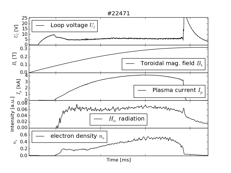
shot_no = 22471
identifier = "loop_voltage"
# create data cache in the 'golem_cache' folder
ds = np.DataSource('golem_cache')
#Create a path to data and download and open the file
base_url = "http://golem.fjfi.cvut.cz/utils/data/"

def get_data(identifier):
    data_file = ds.open(base_url+ str(shot_no) + '/' + identifier)
    return np.loadtxt(data_file)

fig = plt.figure(1)
plt.subplots_adjust(hspace=0.001)

sbp1=plt.subplot(511)
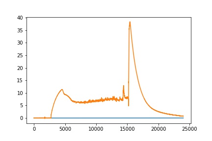
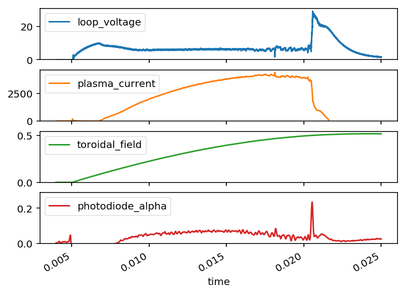
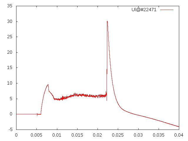
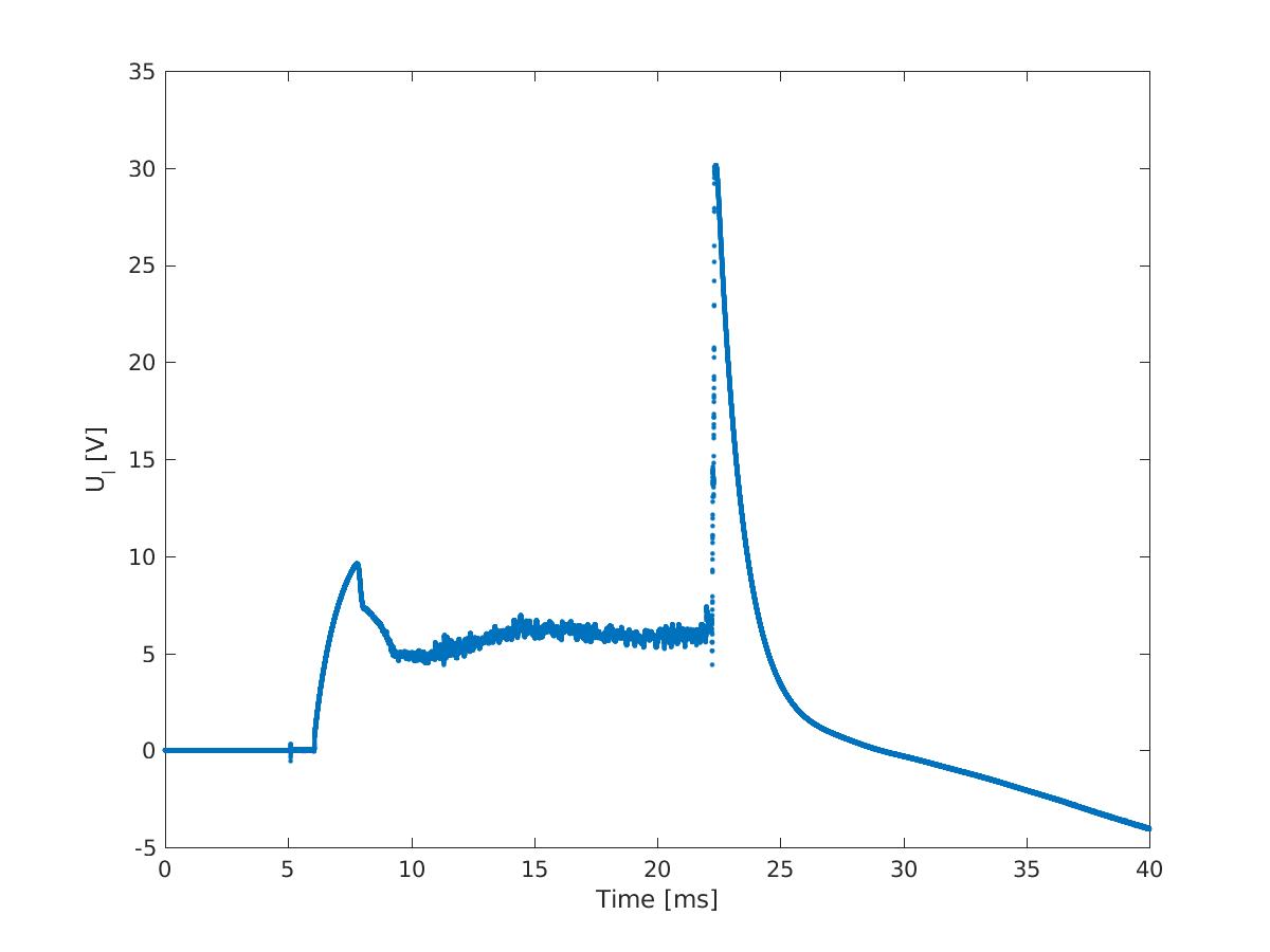
data1 = get_data('loop_voltage')
plt.ylim(0,26)
plt.yticks(np.arange(0, 30, 5))
plt.title('#'+str(shot_no))
plt.ylabel('$U_l$ [V]')
plt.plot(data1[:,0]*1000, data1[:,1], 'k-',label='Loop voltage $U_l$' )
plt.legend(loc=0)

sbp1=plt.subplot(512, sharex=sbp1)
data2 = get_data('toroidal_field')

plt.yticks(np.arange(0, 0.5 , 0.1))
plt.ylim(0,0.35)
plt.ylabel('$B_t$ [T]')
plt.plot(data2[:,0]*1000, data2[:,1], 'k-',label='Toroidal mag. field $B_t$')
plt.legend(loc=0)

sbp1=plt.subplot(513, sharex=sbp1)
data3 = get_data('plasma_current')
plt.yticks(np.arange(0, 4.5, 1))
plt.ylim(0,4.5)
plt.ylabel('$I_p$ [kA]')
plt.plot(data3[:,0]*1000, data3[:,1]/1000, 'k-',label='Plasma current $I_p$')
plt.legend(loc=0)

sbp1=plt.subplot(514, sharex=sbp1)
data4 = get_data('photodiode_alpha')
plt.yticks(np.arange(0, 0.09 , 0.02))
plt.ylim(0,0.09)
plt.ylabel('Intensity [a.u.]')
plt.plot(data4[:,0]*1000, data4[:,1], 'k-',label='$H_\\alpha$ radiation')
plt.legend(loc=0)

sbp1=plt.subplot(515, sharex=sbp1)
data5 = get_data('electron_density')
plt.yticks(np.arange(0, 0.8 , 0.2))
plt.ylim(0,0.8)
plt.ylabel('$n_e$')
plt.xticks(np.arange(8, 30, 5))
plt.xlim(5,25)
plt.xlabel('Time [ms]')
plt.plot(data5[:,0]*1000, data5[:,1]*1e-19, 'k-',label='electron density $n_e$')
plt.legend(loc=0)

xticklabels = sbp1.get_xticklabels()
plt.setp(xticklabels, visible=False)

plt.savefig('basicgraph.pdf')
plt.savefig('basicgraph.jpg')

plt.show()