Diagnostics based on magnetic coils are presently the standard method for measuring magnetic fields in tokamak experiments. Coils are (in the first approximation) easy to manufacture, simple to implement and straightforward to interpret. However, as usual, things get more complicated in a detailed view. The most important requirements which every useful probe-type diagnostic must satisfy are:

• reasonable sensitivity (signal-to-noise ratio); the probe must provide signal high enough to overcome the electronic noise associated with impulse devices
• a good frequency response, so as to follow the most rapid fluctuations present in the system
• minimum perturbing effect on plasma, which means the smallest possible size and appropriate vacuum-friendly and plasma-resistant construction materials

It is unfortunate that these requirements conflict directly with each other. To improve the frequency response (collect high frequencies without attenuation), the coil should be as small as possible. However, small effective area means small signal and bad signal-to-noise ratio.

#Theory of magnetic field measurement using coils

Technically measuring coils do not measure magnetic field itself; they measure the time changes of the magnetic field. (As a result, coils do not measure stationary magnetic field.) More precisely, they react to the time derivative of the magnetic flux \(\Phi\) passing through their turns by inducing a voltage \(U_\mathrm{p}\) upon itself.

\[ U_\mathrm{p} = - \frac{\mathrm{d}\Phi}{\mathrm{d}t} \]

The magnetic flux \(\Phi\) [Wb] passing through a single loop is defined as \[ \Phi = \int_{A_{\mathrm{loop}}} \textbf{B} \cdot \mathrm{d}\textbf{A} \] where \(A_{loop}\) is the loop area. If the loop is small enough to consider the magnetic field \(\textbf{B}\) inside it uniform, we may simplify the formula to \[ \Phi = B_\perp A_{\mathrm{loop}} \] where \(B_\perp\) is the magnetic field component perpendicular to the loop. Now since a coil typically has \(N\) turns, the voltages induced on top of them stack. Denoting the coil effective area \(A_{\mathrm{eff}} = N A_{\mathrm{loop}}\), we may write \[ U_\mathrm{p} = - A_{\mathrm{eff}} \frac{\mathrm{d}B_\perp}{\mathrm{d}t}. \] Finally the coil is typically oriented so that the measured magnetic field is perpendicular to its turns; that is, the coil axis lies parallel to the magnetic field. For instance, a coil measuring the toroidal magnetic field \(B_T\) will be oriented in the toroidal direction. Under this assumption we may finally write \[ U_\mathrm{p} = - A_{\mathrm{eff}} \frac{\mathrm{d}B}{\mathrm{d}t} \] where \(B\) is the measured magnetic field.

Circuit scheme

The following figure shows a simplified scheme of a measuring coil circuit.

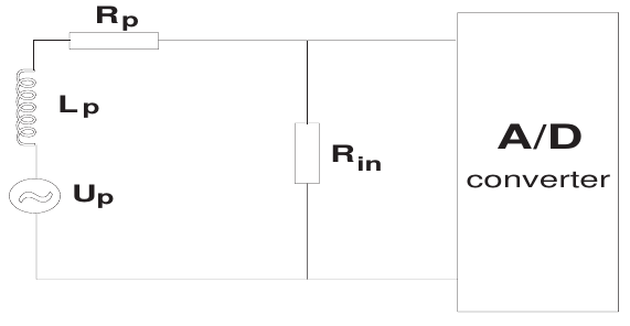
The coil is represented by the parameters with the subscript \(p\): the induced voltage \(U_p\), the inductance \(L_p\) and the resistance \(R_p\). \(R_{in}\) is the input resistance of the analog-to-digital (A/D) converter. In a standard configuration \(R_{in} \ll R_p\).

Coil signal processing

Integration

To extract the magnetic field \(B\) from the measured quantity (\(U_p\)), the coil signal must be integrated. The integration can be either analog or digital.

Analog integration can be performed with passive (RC-like integrating) or with active elements (transistors). Passive integration is more transparent but it requires additional circuits, which lowers the output signal significantly. Conversely, active integration combined with amplification provides a stronger signal, but the additional active elements complicate the data interpretation and for longer time periods (\(\sim 1000 \mathrm{s}\)) integrator drifts can present a serious complication.

The alternative is digital integration; that is, to digitize the coil output directly and perform the integration numerically on a computer. This is the simplest option if the integrated signal is not needed in real-time, as it requires no additional circuits and the signal-to-noise ration is typically good (depending on the coil properties). Since data processing tools are readily available on GOLEM, we use this method for all coil measurements. One is of course limited by the finite resolution of the A/D converters.

Digital integration may be performed, for instance, with the following code:

// input and output arrays
values[LENGTH]  //array of raw data from magnetic coil (input)
B_tor[LENGTH]   //the magnitude of the magnetic field will be written in this array (output)

//magnetic coil's constants
DELTA_T         //time between two samples (1Mhz = 1e-6s, 100kHz = 1e-5s)
CALIBRATION     //calibration constant to convert the voltage to magnetic field

integr = 0
for (i = 0; i <<<> LENGTH; i++)
{
   integr += values[i]
   B_tor[i] = integr * DELTA_T * CALIBRATION
}

Offset removal

An offset is a non-physical addition to a signal, created by noise in the electronics, parasitic voltages, cross-talk between the diagnostics and many other influences. The figure above demonstrates the impact an offset can have on data integration. In blue, the real, physical \(dB/dt\) and \(B\) are plotted. In red, a small constant offset was added to the entire raw signal. In green, a normal-distributed noise with a zero mean was added to the raw signal. One observes the effect that this has on the integrated signal, in particular the in the red case.

In every magnetic measurement, offsets are more than likely to appear on the collected voltage signals. The simplest method to remove them is to average the first few hundred/thousands of samples (before the 5 ms mark when GOLEM discharges begin) and subtract this average from the signal prior to its integration. This method will fail if the offset is time-dependent, in which case more advanced methods are required [link].

Diagnostics based on magnetic coils

• Toroidal Magnetic field
• Mirnov coils at limiter

Note: Excerpt from I. Ďuran: Fluctuations of magnetic field in the CASTOR tokamak, Dissertation Thesis, 2003